Ebisu, a recently launched protocol, introduces an interesting opportunity for DeFi investors: the ability to borrow against sUSDe at a fixed rate. This offers predictability, but also comes with a key risk: setting your borrow rate too low risks redemption, where both collateral and debt are liquidated.

In this article, we explore the question: Where should investors set their fixed borrow rate to maximise returns while avoiding redemption over one year without adjusting their position?

Simulating Market Conditions

Before running any strategy tests, we first need a realistic representation of market conditions for stablecoins.

To achieve this, we base our simulations on the 512M Stablecoin Prime Rate (SPR), a TVL-weighted APY index of the largest stablecoin pools in DeFi. This index captures global stablecoin demand trends.

Using the SPR, we establish a statistical relationship between it and the yield on sUSDe. As in our previous dTRINITY analysis, we employ a Gradient Boost Regression model to map this relationship. The results of which are shown below.

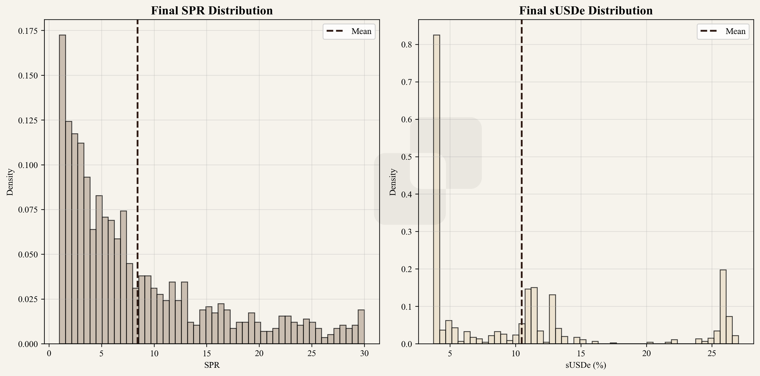
Next, we use historical SPR data to generate a distribution of possible values through bootstrapping. This technique resamples the existing data (around 1.5 years of observations) to create thousands of hypothetical outcomes. We run 2,000 simulated paths for the SPR. Applying our Gradient Boost model to these simulated SPR paths yields the corresponding sUSDe yield paths. Both sets of simulations are illustrated in the figure below.

While this is a simplified approach, limited by the relatively short historical record, it provides a reasonable basis for scenario testing. The resulting final distributions for both SPR and sUSDe yields are summarised in the figure below.

Determining the Minimum Viable Borrow Rate

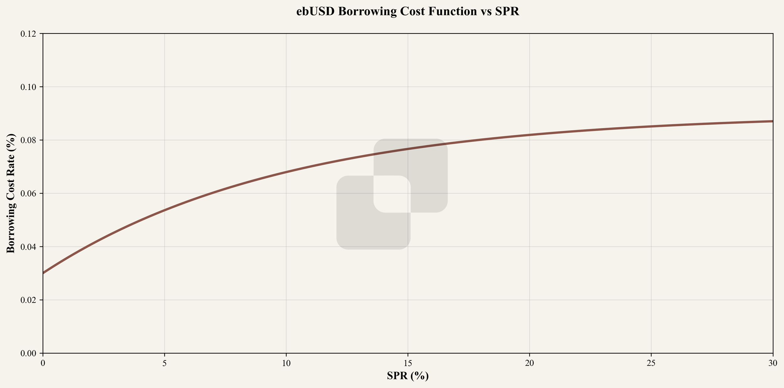
A crucial input is the minimum viable fixed borrow rate on Ebisu, which we derive from the SPR. This is done using an exponential function modelled after the behaviour observed in Liquity V2 since its launch.

The logic is straightforward: as market demand for stablecoins increases (and the SPR rises), the rates for borrowing, fixed or otherwise, also rise. However, this relationship is not linear. At higher SPR values, the index reflects not only borrowing rates but also yields from DEX LPs, off-chain lending, and other sources.

The result of this modelling is shown below, representing the theoretical lowest possible fixed borrow rate before redemption risk becomes significant.

Simulating the Strategy

To test how different fixed borrowing rates perform in practice, we set up a simulation with the following parameters:

Starting portfolio: 1,000 sUSDe.
Borrowing: ebUSD at a 90% loan-to-value (LTV) ratio.
Leverage limit: Maximum of 5× to prevent excessive compounding risk.
Fixed borrow rate: Expressed as a multiplier of the Redemption Borrow APY, ranging from 1.2× to 2.4× in 0.1 increments.
Market & execution assumptions: Perfect liquidity, no transaction costs, and no slippage.
Time horizon: 365 days, with no position adjustments once initiated.

The objective is to see how long a position can survive without redemption and how the total return profile changes as the fixed borrow rate is varied.

Redemption Rates and Cumulative Returns

The left graph in the figure below plots the probability of redemption for each fixed-rate multiplier. At the lower end (1.2×–1.5×), redemption risk is significant: many simulated paths see the loan being liquidated before the year is up. This happens because the fixed rate is only slightly above the Redemption Borrow APY, leaving little cushion if market rates rise or collateral yields fall.

As the multiplier increases, the redemption probability falls sharply. Around the 2.2× mark, the curve flattens at zero, meaning none of the simulated paths result in a redemption event. This threshold is critical: it marks the point where a fixed rate is high enough to survive even the worst-case scenarios in our simulated yield environment.

The right graph in the figure above shows how the mean cumulative returns change with the rate multiplier. At low multipliers, returns are suppressed because frequent redemptions cut positions short, crystallising losses and eliminating the chance for compounding.

As the redemption probability decreases (around 1.8×–2.1×), mean returns begin to climb, benefiting from more prolonged position survival and stable yield generation. The real inflexion point comes at 2.2×, where redemptions drop to zero, with mean cumulative returns jumping sharply as all simulations now run the whole year without interruption. Beyond this, returns level off, as the higher fixed rate slightly reduces net yield.

Heatmap Analysis

The heatmap shown below offers a more intuitive view of the relationship between the fixed rate multiplier and the strategy’s overall performance. At the lower end of the multiplier range, the chart is dominated by darker shades, reflecting the consistently poor outcomes caused by frequent redemptions. As the multiplier increases, these dark tones gradually give way to lighter colours, signalling more substantial returns as positions survive longer and benefit from uninterrupted yield generation.

A clear visual break occurs at the 2.2× multiplier, where the entire column shifts into noticeably lighter and redder shades. This marks the point at which redemption events disappear entirely and the strategy delivers consistently higher returns across all simulated market paths. The heatmap, therefore, not only confirms the trends seen in previous figures but also provides an immediate visual cue for identifying the optimal threshold.

Conclusion and Limitations

This analysis underscores the delicate balance between maximising returns and avoiding redemption risk when looping sUSDe with a fixed borrow rate on Ebisu. For passive investors unwilling to monitor or adjust their positions over a year, a fixed rate set at around 2.2× the Redemption Borrow APY appears optimal in our simulations. At this level, the strategy benefits from uninterrupted compounding while eliminating the risk of forced liquidation.

However, this approach is not necessarily the most profitable for active managers. By selecting a lower fixed rate and making periodic adjustments, it is possible to capture higher yields while still keeping redemption risk under control. The trade-off lies in the time and attention required, as well as the execution risk that comes with more frequent rebalancing. Automation tools such as IR-managers can help bridge this gap, dynamically adjusting borrowing parameters to preserve safety while maximising returns.

It is essential to know the limitations of this article. The historical data for both sUSDe and the SPR spans only around one and a half years, which constrains the robustness of the statistical modelling. The simulation also assumes perfect liquidity and the absence of transaction costs. Furthermore, real-world performance could be affected by unexpected factors such as liquidity shortages, oracle delays, or protocol-level changes. These caveats mean that while the findings provide a helpful guide for fixed-rate strategy design, they should be applied with caution and adapted to evolving market conditions.

This article may contain material that is not directed to, or intended for distribution to or use by, any person or entity who is a citizen or resident of or located in any locality, state, country or other jurisdiction where such distribution, publication, availability or use would be contrary to law or regulation or which would subject 512m AG or its affiliates to any registration or licensing requirement within such jurisdiction. The information, tools and material presented in this article are provided to you for information purposes only and are not to be used or considered as an offer or the solicitation of an offer to sell or to buy or subscribe for securities or other financial instruments.

Optimising Returns on Ebisu